Unit Cube
Overview
A very simple unit cube example intended for learning the basic aspects of OpenPAME like config files, case structure and data handling. It also helps the developers to debugging the code.
The mesh consists only of 6 panels. The cube has a dimension of 1x1x1 units. As OpenPAME expects all units to be in SI units, a geometrical dimension with 1 unit is equal to 1 meter.
Updates
Starting from OpenPAME version 0.5.3 we make use of the so called coMesh concept. This means all the different needed meshes like wake, the main mesh, the input mesh and all other go into seperate directories. So the newest case structure looks like this
cube
├───0
├───base
│   └───0
│       └───mesh
└───config
while the input mesh is now placed into cube\base\0\mesh instead of cube\0\mesh as prior to version 0.5.3. All the mesh files are assumed to be named mesh.fsi.gz for the internal mesh format.
Case Setup
This example assumes the mesh is already imported and prepared so we can start configuring the case. So first lets have an overview to the configuration files. OpenPAME has for most of the logic units a separate config file. All the config files go into the config directory, obviously.
Config files
Here is an overview of all the config files needed for the current OpenPAME version. Important Note: While OpenPAME is under active development changes to the configuration files may occur at any time!
axisSetup
cleanUpCase
coMesh
createFields
interpolationSchemes
panelMethod
parallel
runTime
solvers
wakeSetup
We will now go through all the most important config files, while leaving out files a normal user would not need to change for now. Side Note: all the config files are based on lua and might be scripted by the user.
runTime config file
This is one of the main config files so far. Here you can define the number of outer iterations or time steps and the time step size if you want. Also you can specifiy the sequence the results will be written and some other in-/output aspects of the simulations. This is what it looks like, pretty self explanatory so.
-- runTime config file

--
-- the time folder the simulation should start from
--
startTime = 0

--
-- the end time for the simulation
--
endTime = 1

--
-- the time step size
--
deltaT = 1

--
-- the sequence number for writing results
--
autoSaveIter = 1

--
-- the precision for the ascii result files
--
precision = 6

--
-- switch on compatibility mode for older OpenPAME versions
--
compatible = true

--
-- use binary io for storing the matrices
--
binary = false
axisSetup config file
This config file simply defines the orientation of the geometry regarding pitch-, yaw- and roll axis. This is needed to determine the lift and drag force direction and also to find the trailing edges.
-- specification of the global coordinate system

--
-- the roll axis definition
--
rollAxis  = fsi.point( 1.0, 0.0, 0.0 );

--
-- the pitch axis definition
--
pitchAxis = fsi.point( 0.0, 1.0, 0.0 );
wakeSetup config file
This config file is used for configuring the modeling of the wake mesh. It also demonstrates a simple scripting through including other config files and using their variables to calculate dependent variables.
-- wake calculation procedure

--
-- include some other config files for reference values
--
dofile "config/panelMethod"
dofile "config/runTime"

--
-- reference trailing edge normal angle / ( degree )
-- desribes the angle between the normal of two faces
-- must not be less than 100 degree
--
trailingEdgeAngle = 120

--
-- wakeDelta / ( m )
--
wakeDelta = qMag * deltaT

--
-- wakeAngleFactor / ( true or false )
--
-- enter true for using specific wake (runs along trailing edge direction)
-- enter false for using standard wake (runs along rolLAxis direction)
--
specificWake = false

--
-- wakeAngleFactor = -0.5 : wake runs along the upper side of airfoil
-- wakeAngleFactor = 0 : wake runs along half of the trailing edge angle (default mode)
-- wakeAngleFactor = 0.5 : wake runs along the lower side of airfoil
--
wakeAngleFactor = 0

--
-- yaw edge angle / ( deg )
-- if angle between trailing edge vector and yaw is greater than it
-- it will become a trailing edge, otherwise it will left untouched
-- usefull for vertical tail exclusion
--
yawEdgeAngle = 0
panelMethod config file
This is the configuration file specific to the implemented panel method.
-- panelMethod config file

--
-- the angle of attack / ( deg )
--
AoA = 0.0
rAoA = math.pi * AoA / 180.0

--
-- the inflow velocity / ( m/s )
--
qMag = 5.0
--
qInfty = fsi.point( qMag * math.cos(rAoA), 0.0, qMag * math.sin(rAoA) )

--
-- reference density / ( kg / m^-3 )
--
rhoRef = 1.2041

--
-- reference pressure / ( Pa )
--
pRef = 101325

--
-- reference Temperature / ( degC )
--
TRef = 20

--
-- kappa / ( 1 )
--
kappa = 1.4

--
-- R (gas constant) / ( J / ( kg K ) )
--
R = 287

--
-- height / ( m )
--
H = 0

--
-- reference Area for coefficient calculation / ( m^2 )
--
refArea = 6
cleanUpCase config file
The last config file in this example is the cleanUpCase file. This file is specific to a cleanUpCase application which removes, after running the simulation, all created files and keeps only files that are protected. This is usefull in the case you want to rerun the simulation and need to get rid of all old results for example.
-- cleanUpCase config file

--
-- some global variables
--
keepEpmtyDirs = false
confirmAction = false
verbose = false

--
-- definition of files and dirs to protect
--
protected = {

  -- the dirs
  dirs = {
    "0",
    "base/0/mesh",
    "config",
  },

  -- the files
  files = {
    "base/0/mesh/mesh.fsi.gz",
    "rerun.bat",
    "run.bat",
    "clean.bat",
    "config/solvers",
    "config/runTime",
    "config/parallel",
    "config/panelMethod",
    "config/interpolationSchemes",
    "config/createFields",
    "config/cleanUpCase",
    "config/wakeSetup",
    "config/axisSetup",
    "config/coMesh",
  }
}
Preprocessing steps
Now the case is setup and we can proceed with the steps to initialize the simulation to get the job running.
setupPanelMethod
Importand Note: this application is under investigation to split it in some more seperate steps, so please be warned: This step might change in the near future.
Change on the command line into the case directory and run the application:
[cube]$ setupPanelMethod
Now you chould see an output like this:
 ____  ____   __
(  __)/ ___) (  )
 ) _) \___ \  )(  v0.5.3RC1
(__)  (____/ (__) FrameWork

executable  : setupPanelMethod
working dir : /home/rt/run/tutorials/solver/panelMethod/cube
install dir : /home/rt/devel/fsi/bin/setupPanelMethod
time        : 2020-Jul-08 14:54:02

parallel execution is off.
reading axis setup config
the roll axis is located in direction ( 1 0 0 )
the pitch axis is located in direction ( 0 1 0 )
the yaw axis is located in direction ( 0 0 1 )

creating baseCoMesh
8 nodes, 0 edges, 6 faces, 0 cells read in.
creating surfaceMesh from coMesh
creating empty wakeCoMesh
creating empty wakeMesh from coMesh

reading system config
  reference normal angle of trailing edge: 120 degree
  yaw edge tolerance angle: 0 degree
  wakeDelta: 5 m
  specific wake: false
  wakeAngleFactor: 0

get trailing edge(s)
  no trailing edge found

writing zone included body mesh
8 nodes, 0 edges, 6 faces, 0 cells written.

wall : 0.00784s
user : 0.00000s
sys  : 0.01000s

done.
Checking the directory structure shows that the mesh object in cube/0/mesh was created (compare it to the clean structure) and we can now proceed with the calculation of the system matrices for the panel method.
cube
├───0
│   └───mesh
├───base
│   └───0
│       └───mesh
└───config
calcPanelCoeff
Change on the command line into the case directory and run the application:
[cube]$ calcPanelCoeff
You should see a similiar output:
 ____  ____   __
(  __)/ ___) (  )
 ) _) \___ \  )(  v0.5.3RC1
(__)  (____/ (__) FrameWork

executable  : calcPanelCoeff
working dir : /home/rt/run/tutorials/solver/panelMethod/cube
install dir : /home/rt/devel/fsi/bin/calcPanelCoeff
time        : 2020-Jul-08 15:04:25

parallel execution is off.
creating runTime.

startTime : 0
endTime   : 1
deltaT    : 1

reading axis setup config
the roll axis is located in direction ( 1 0 0 )
the pitch axis is located in direction ( 0 1 0 )
the yaw axis is located in direction ( 0 0 1 )

creating surfaceMesh at time = 0
8 nodes, 0 edges, 6 faces, 0 cells read in.

creating faceVectorSurfaceField normals
creating faceVectorSurfaceField centers

creating body doublet coefficient matrix A
creating body source coefficient matrix B

calculate normals and centers for each face
calculate source and doublet geometry coefficient matrices.

writing body doublet coefficient matrix A to file
writing body source coefficient matrix B to file

writing at Time = 0
8 nodes, 0 edges, 6 faces, 0 cells written.
  vectorSurfaceMeshField face centers
  vectorSurfaceMeshField face normals


wall : 0.02144s
user : 0.00000s
sys  : 0.01000s

done.
Again check the directory structure and some new directories and files are created. There are some first fields (faceVectorFields) created in cube/0/vectorField/face and the system matrices are stored in cube/matrices.
├───0
│   ├───mesh
│   └───vectorField
│       └───face
├───base
│   └───0
│       └───mesh
├───config
└───matrices
Now all preprocessing steps are done, we can forward to the simulation.
Running the simulation
panelMethod
If you are not already in the case directory change into it and run panelMethod.
[cube]$ panelMethod
This is the output you should see now:
 ____  ____   __
(  __)/ ___) (  )
 ) _) \___ \  )(  v0.5.3RC1
(__)  (____/ (__) FrameWork

executable  : panelMethod
working dir : /home/rt/run/tutorials/solver/panelMethod/cube
install dir : /home/rt/devel/fsi/bin/panelMethod
time        : 2020-Jul-08 15:15:48

parallel execution is off.
creating runTime.

startTime : 0
endTime   : 1
deltaT    : 1

reading axis setup config
the roll axis is located in direction ( 1 0 0 )
the pitch axis is located in direction ( 0 1 0 )
the yaw axis is located in direction ( 0 0 1 )

creating surfaceMesh at time = 0
8 nodes, 0 edges, 6 faces, 0 cells read in.

creating faceScalarSurfaceField sources
creating faceScalarSurfaceField rhs
creating faceScalarSurfaceField doublets
creating faceScalarSurfaceField u
creating faceScalarSurfaceField v
creating faceScalarSurfaceField w
creating faceScalarSurfaceField pressure
creating faceScalarSurfaceField p_abs
creating faceScalarSurfaceField machNumber
creating faceScalarSurfaceField Cp
creating faceVectorSurfaceField velocity
creating faceVectorSurfaceField force
creating faceVectorSurfaceField centers
creating faceVectorSurfaceField normals
creating faceVectorSurfaceField gradDoublets

reading body doublet coefficient matrix A from file
reading body source coefficient matrix B from file

reading system config
  inflow velocity: 5 m/s
  angle of attack: 0 degree
  air density: 1.2041 kg/m^3
  reference pressure: 101325 Pa
  temperature: 293.15 K
  height: 0 m
  reference area: 6 m^2

(1/1) - Time : 1 sec.
solve equation system for current time step

PBiCGSTAB: solve doublets, initial residual = 1, final residual = 0, iterations = 0
solve time: wall = 0.005s, user = 0.000s, sys = 0.000s
final iteration, no relaxation.

reconstruct velocity field
  sonic speed = 343.2 m/s
  percentage of faces in subsonic range ( Mach < 0.8 ): 100 %
  percentage of faces in transsonic range ( 0.8 < Mach < 1.2 ): 0 %
  percentage of faces in supersonic range ( Mach > 1.2 ): 0 %
reconstruct pressure field
reconstruct forces
  global forces
    ( +0.00000e+00 +0.00000e+00 +0.00000e+00 ) [N], mag: +0.00000e+00 [N] : total
    ( +0.00000e+00 +0.00000e+00 +0.00000e+00 ) [N], mag: +0.00000e+00 [N] : lift
    ( +0.00000e+00 +0.00000e+00 +0.00000e+00 ) [N], mag: +0.00000e+00 [N] : drag
  partial forces
    ( +0.00000e+00 +0.00000e+00 +0.00000e+00 ) [N], mag: +0.00000e+00 [N] : lowerTE
    ( +0.00000e+00 +0.00000e+00 +0.00000e+00 ) [N], mag: +0.00000e+00 [N] : upperTE
reconstruct the aerodynamic coefficients
  calculate pressure coefficient distribution
  lift coefficient: Cl = +0.000e+00
  drag coefficient: Cd = +0.000e+00

writing autosave at Time = 1
8 nodes, 0 edges, 6 faces, 0 cells written.
  scalarSurfaceMeshField face Cp
  scalarSurfaceMeshField face Mach
  scalarSurfaceMeshField face doublets
  scalarSurfaceMeshField face p_abs
  scalarSurfaceMeshField face pressure
  scalarSurfaceMeshField face rhs
  scalarSurfaceMeshField face sources
  scalarSurfaceMeshField face u
  scalarSurfaceMeshField face v
  scalarSurfaceMeshField face w
  vectorSurfaceMeshField face F
  vectorSurfaceMeshField face centers
  vectorSurfaceMeshField face gradDoublets
  vectorSurfaceMeshField face normals
  vectorSurfaceMeshField face velocity

wall : 0.06366s
user : 0.00000s
sys  : 0.00000s

done.
Again checking the directory structure you see there is a new time folder cube/1 containing a mesh and different faceScalar- and faceVectorFields. This are the simulation results.
cube
├───0
│   ├───mesh
│   └───vectorField
│       └───face
├───1
│   ├───mesh
│   ├───scalarField
│   │   └───face
│   └───vectorField
│       └───face
├───base
│   └───0
│       └───mesh
├───config
└───matrices
Now you have done your first OpenPAME simulation. Please be aware of the forces and coefficients in the output and try to explain why this are the correct values for the panelMethod. now lets proceed to the post processing.
Post processing
For Postprocessing you might be interested in cp distributions. This is work in progress. What you can already do is to convert the results into some formats a post processor can read in. All you have to do is to choose a result export fitting your needs.
results2legacyVTK
In this case we will use the export to legacy VTK format.
[cube]$ results2legacyVTK
The output:
 ____  ____   __
(  __)/ ___) (  )
 ) _) \___ \  )(  v0.5.3RC1
(__)  (____/ (__) FrameWork

executable  : results2legacyVTK
working dir : /home/rt/run/tutorials/solver/panelMethod/cube
install dir : /home/rt/devel/fsi/bin/results2legacyVTK
time        : 2020-Jul-08 15:30:15

parallel execution is off.
creating runTime.

startTime : 0
endTime   : 1
deltaT    : 1

timeloop start.
creating Mesh at time = 0
8 nodes, 0 edges, 6 faces, 0 cells read in.

8 nodes, 0 edges, 6 faces, 0 cells written.

0/vector/face: centers, normals,

creating Mesh at time = 1
8 nodes, 0 edges, 6 faces, 0 cells read in.

8 nodes, 0 edges, 6 faces, 0 cells written.

1/scalar/face: Cp, Mach, doublets, p_abs, pressure, rhs, sources, u, v, w,
1/vector/face: F, centers, gradDoublets, normals, velocity,

wall : 0.06284s
user : 0.00000s
sys  : 0.02000s

done.
Checking the directory structure shows a new directory vtk is created. There you will find a VTK file for each timestep.
cube
├───0
│   ├───mesh
│   └───vectorField
│       └───face
├───1
│   ├───mesh
│   ├───scalarField
│   │   └───face
│   └───vectorField
│       └───face
├───base
│   └───0
│       └───mesh
├───config
├───matrices
└───vtk
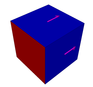
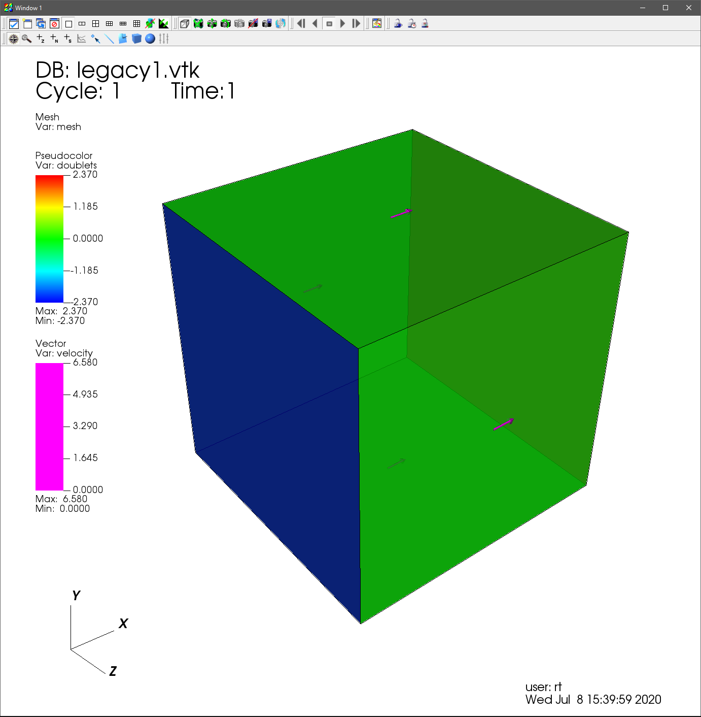
Postprocessor
The exported VTK files might be read in by any Postprocessor like FieldView, VisIt or ParaView and others. You can make some nice plots and screenshots if needed. In our case VisIt is used.
cleanUpCase
Now you might want to play around with this example you want to delete all the created files. Simply running
[cube]$ cleanUpCase
outputs:
 ____  ____   __
(  __)/ ___) (  )
 ) _) \___ \  )(  v0.5.3RC1
(__)  (____/ (__) FrameWork

executable  : cleanUpCase
working dir : /home/rt/run/tutorials/solver/panelMethod/cube
install dir : /home/rt/devel/fsi/bin/cleanUpCase
time        : 2020-Jul-08 15:50:52

parallel execution is off.
setting up case structure.

path is: /home/rt/run/tutorials/solver/panelMethod/cube

number of directories found: 16
number of directories protected: 3
number of directories to delete: 13

number of files found: 38
number of files protected: 14
number of files to delete: 27

wall : 0.08204s
user : 0.00000s
sys  : 0.08000s

done.
and the directory structure should look like at the start of this example.
cube
├───0
├───base
│   └───0
│       └───mesh
└───config
Summary
Now you have learned the basic steps to do a simulation with OpenPAME. The important configuration files, the needed applications and how to get the postprocessing done.
